Hydraulic calculation of a one-pipe and two-pipe heating system with formulas, tables and examples
The cost-effectiveness of thermal comfort in the house is ensured by the calculation of hydraulics, its high-quality installation and proper operation. The main components of the heating system are a heat source (boiler), a heat main (pipes) and heat transfer devices (radiators). For efficient heat supply, it is necessary to maintain the initial parameters of the system at any load, regardless of the season.
Before starting hydraulic calculations, perform:
- Collection and processing of information on the object in order to:
- determining the amount of heat required;
- choice of heating scheme.
- Thermal calculation of the heating system with justification:
- volumes of thermal energy;
- loads;
- heat loss.
If water heating is recognized as the best option, a hydraulic calculation is performed.
To calculate hydraulics using programs, familiarity with the theory and laws of resistance is required. If the formulas below seem difficult to understand, you can choose the options that we offer in each of the programs.
The calculations were carried out in the Excel program. The finished result can be seen at the end of the instructions.
Determination of the number of gas control points of hydraulic fracturing
Gas control points are designed to reduce gas pressure and maintain it at a given level, regardless of the flow rate.
With a known estimated consumption of gaseous fuel, the city district determines the number of hydraulic fracturing, based on the optimal hydraulic fracturing performance (V=1500-2000 m3/hour) according to the formula:
n = , (27)
where n is the number of hydraulic fracturing, pcs.;
VR — estimated gas consumption by the city district, m3/hour;
Vwholesale — optimum productivity of hydraulic fracturing, m3/hour;
n=586.751/1950=3.008 pcs.
After determining the number of hydraulic fracturing stations, their location is planned on the general plan of the city district, installing them in the center of the gasified area on the territory of the quarters.
Program overview
For the convenience of calculations, amateur and professional programs for calculating hydraulics are used.
The most popular is Excel.
You can use the online calculation in Excel Online, CombiMix 1.0, or the online hydraulic calculator. The stationary program is selected taking into account the requirements of the project.
The main difficulty in working with such programs is ignorance of the basics of hydraulics. In some of them, there is no decoding of formulas, the features of branching of pipelines and the calculation of resistances in complex circuits are not considered.
- HERZ C.O. 3.5 - makes a calculation according to the method of specific linear pressure losses.
- DanfossCO and OvertopCO can count natural circulation systems.
- "Flow" (Flow) - allows you to apply the calculation method with a variable (sliding) temperature difference along the risers.
You should specify the data entry parameters for temperature - Kelvin / Celsius.
What is hydraulic calculation
This is the third stage in the process of creating a heating network. It is a system of calculations that allows you to determine:
- diameter and throughput of pipes;
- local pressure losses in the areas;
- hydraulic balancing requirements;
- system-wide pressure losses;
- optimal water flow.
According to the data obtained, the selection of pumps is carried out.
For seasonal housing, in the absence of electricity in it, a heating system with natural circulation of the coolant is suitable (link to review).
The main purpose of the hydraulic calculation is to ensure that the calculated costs for the circuit elements coincide with the actual (operational) costs. The amount of coolant entering the radiators should create a heat balance inside the house, taking into account the outside temperatures and those set by the user for each room according to its functional purpose (basement +5, bedroom +18, etc.).
Complex tasks - cost minimization:
- capital - installation of pipes of optimal diameter and quality;
- operational:
- dependence of energy consumption on the hydraulic resistance of the system;
- stability and reliability;
- noiselessness.

Replacing the centralized heat supply mode with an individual one simplifies the calculation method
For autonomous mode, 4 methods of hydraulic calculation of the heating system are applicable:
- by specific losses (standard calculation of pipe diameter);
- by lengths reduced to one equivalent;
- according to the characteristics of conductivity and resistance;
- comparison of dynamic pressures.
The first two methods are used with a constant temperature drop in the network.
The last two will help distribute hot water to the rings of the system if the temperature drop in the network no longer matches the drop in risers / branches.
Overview of programs for hydraulic calculations

Sample program for heating calculation
In fact, any hydraulic calculation of water heating systems is a complex engineering task. To solve it, a number of software packages have been developed that simplify the implementation of this procedure.
You can try to make a hydraulic calculation of the heating system in the Excel shell, using ready-made formulas. However, the following problems may occur:
- Big error. In most cases, one-pipe or two-pipe schemes are taken as an example of a hydraulic calculation of a heating system. Finding such calculations for the collector is problematic;
- To correctly account for the hydraulic resistance of the pipeline, reference data is required, which are not available in the form. They need to be searched and entered additionally.
Given these factors, experts recommend using programs for calculation. Most of them are paid, but some have a demo version with limited features.
Oventrop CO

Program for hydraulic calculation
The simplest and most understandable program for the hydraulic calculation of the heat supply system. An intuitive interface and flexible settings will help you quickly deal with the nuances of data entry. Small problems may arise during the initial setup of the complex. It will be necessary to enter all the parameters of the system, starting from the pipe material and ending with the location of the heating elements.
It is characterized by flexibility of settings, the ability to make a simplified hydraulic calculation of heating both for a new heat supply system and for upgrading an old one. Differs from analogues in a convenient graphical interface.
Instal-Therm HCR
The software package is designed for professional hydraulic resistance of the heat supply system. The free version has many limitations. Scope - design of heating in large public and industrial buildings.
In practice, for autonomous heat supply of private houses and apartments, hydraulic calculation is not always performed. However, this can lead to a deterioration in the operation of the heating system and the rapid failure of its elements - radiators, pipes and a boiler. To avoid this, it is necessary to calculate the system parameters in a timely manner and compare them with the actual ones in order to further optimize the heating operation.
An example of a hydraulic calculation of a heating system:
Verification hydraulic calculation of the gas pipeline branch
The purpose of the calculation: Checking the pressure at the inlet to the gas distribution station.
Initial data:
table
|
Throughput, qday, million m3/day |
8,4 |
|
Initial pressure of the gas pipeline section, Рn , MPa |
2,0 |
|
Final pressure of the gas pipeline section, Рк , MPa |
1,68 |
|
Length of the gas pipeline section, L, km |
5,3 |
|
Diameter of the gas pipeline section, dn x, mm |
530 x 11 |
|
Average annual soil temperature at the depth of the gas pipeline, tgr, 0C |
11 |
|
Gas temperature at the beginning of the gas pipeline section, tn, 0C |
21 |
|
Heat transfer coefficient from gas to soil, k, W / (m20С) |
1,5 |
|
Heat capacity of gas, cf, kcal/(kg°С) |
0,6 |
|
Gas composition |
Table 1 — Composition and main parameters of gas components of the Orenburg field
|
Component |
Chemical formula |
Concentration in fractions of a unit |
Molar mass, kg/kmol |
Critical temperature, K |
Critical pressure, MPa |
Dynamic viscosity, kgf s/m2x10-7 |
|
Methane |
CH4 |
0,927 |
16,043 |
190,5 |
4,49 |
10,3 |
|
Ethane |
C2H6 |
0,022 |
30,070 |
306 |
4,77 |
8,6 |
|
Propane |
С3Н8 |
0,008 |
44,097 |
369 |
4,26 |
7,5 |
|
Butane |
С4Н10 |
0,022 |
58,124 |
425 |
3,5 |
6,9 |
|
Pentane |
C5H12 |
0,021 |
72,151 |
470,2 |
3,24 |
6,2 |
To perform a hydraulic calculation, we first calculate the main parameters of the gas mixture.
Determine the molecular weight of the gas mixture, M cm, kg / kmol
where а1, а2, аn — volumetric concentration, fractions of units, ;
M1, M2, Mn are the molar masses of the components, kg/kmol, .
Mcm = 0.927 16.043 + 0.022 30.070 + 0.008 44.097 + 0.022 58.124 +
+ 0.021 72.151 = 18.68 kg/kmol
We determine the density of the mixture of gases, s, kg / m3,
where M cm is the molecular weight, kg/mol;
22.414 is the volume of 1 kilomole (Avogadro's number), m3/kmol.
We determine the density of the gas mixture in air, D,
where is the gas density, kg/m3;
1.293 is the density of dry air, kg/m3.
Determine the dynamic viscosity of the gas mixture, cm, kgf s/m2
where 1, 2, n, is the dynamic viscosity of the gas mixture components, kgf s/m2, ;
We determine the critical parameters of the gas mixture, Tcr.cm. , TO
where Тcr1, Тcr2, Тcrn is the critical temperature of the gas mixture components, K, ;
where Pcr1, Pcr2, Pcrn are the critical pressure of the mixture components, MPa, ;
We determine the average gas pressure in the gas pipeline section, Рav, MPa
where Рн is the initial pressure in the gas pipeline section, MPa;
Pk is the final pressure in the gas pipeline section, MPa.
We determine the average gas temperature along the length of the calculated section of the gas pipeline, tav, ° С,
where tn is the gas temperature at the beginning of the calculation section, °С;
dn is the outer diameter of the gas pipeline section, mm;
l is the length of the gas pipeline section, km;
qday is the throughput capacity of the gas pipeline section, million m3/day;
is the relative density of the gas in air;
Cp is the heat capacity of the gas, kcal/(kg°C);
k- coefficient of heat transfer from gas to soil, kcal/(m2h°С);
e is the base of the natural logarithm, e = 2.718.
We determine the reduced temperature and pressure of the gas, Tpr and Rpr,
where Rsr. and Tsr. are the average pressure and temperature of the gas, MPa and K, respectively;
Rcr.cm and Tcr.cm. are the critical pressure and temperature of the gas, MPa and K, respectively.
We determine the coefficient of gas compressibility according to the nomogram depending on Ppr and Tpr.
Z=0.9
To determine the throughput capacity of a gas pipeline or its section in the steady state of gas transport, without taking into account the relief of the route, use the formula, q, million m3 / day,
where din is the internal diameter of the gas pipeline, mm;
Рн and Рк - initial and final pressures of the gas pipeline section, respectively, kgf/cm2;
l is the coefficient of hydraulic resistance (taking into account local resistances along the gas pipeline route: friction, taps, transitions, etc.). It is allowed to take 5% higher than ltr;
D is the relative specific gravity of the gas in air;
Тav is the average gas temperature, K;
? — length of the gas pipeline section, km;
W is the gas compressibility factor;
From formula (4.13) we express Рк, , kgf/cm2,
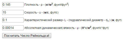
Hydraulic calculation is performed in the following sequence. Determine the Reynolds number, Re,
where qday is the daily throughput capacity of the gas pipeline section, million m3/day;
din is the internal diameter of the gas pipeline, mm;
is the relative density of the gas;
— dynamic viscosity of natural gas; kgf s/m2;
Since Re >> 4000, the mode of gas movement through the pipeline is turbulent, quadratic zone.
The coefficient of friction resistance for all gas flow regimes is determined by the formula, ltr ,
where EC is the equivalent roughness (height of protrusions that create resistance to gas movement), EC = 0.06 mm
We determine the coefficient of hydraulic resistance of the gas pipeline section, taking into account its average local resistances, l,
where E is the coefficient of hydraulic efficiency, E = 0.95.
According to formula (4.14), we determine the pressure at the end of the gas pipeline section.
Conclusion: The obtained pressure value corresponds to the operational one at the final section of the gas pipeline.
Calculation of the hydraulics of the heating system
We need data from the thermal calculation of the premises and the axonometric diagram.
Step 1: count the pipe diameter
As initial data, economically justified results of thermal calculation are used:
1a. The optimal difference between hot (tg) and cooled (to) coolant for a two-pipe system is 20º
1b. Coolant flow rate G, kg/hour — for a one-pipe system.
2. The optimal speed of the coolant is ν 0.3-0.7 m/s.
The smaller the inner diameter of the pipes, the higher the speed. Reaching 0.6 m/s, the movement of water begins to be accompanied by noise in the system.
3. Calculated heat flow rate - Q, W.
Expresses the amount of heat (W, J) transferred per second (unit of time τ):
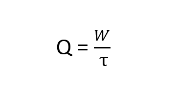
Formula for calculating the heat flow rate
4. Estimated density of water: ρ = 971.8 kg/m3 at tav = 80 °С
5. Plot parameters:
- power consumption - 1 kW per 30 m³
- thermal power reserve - 20%
- room volume: 18 * 2.7 = 48.6 m³
- power consumption: 48.6 / 30 = 1.62 kW
- frost margin: 1.62 * 20% = 0.324 kW
- total power: 1.62 + 0.324 = 1.944 kW
We find the closest Q value in the table:
We get the interval of the inner diameter: 8-10 mm. Plot: 3-4. Plot length: 2.8 meters.
Step 2: calculation of local resistances
To determine the pipe material, it is necessary to compare the indicators of their hydraulic resistance in all parts of the heating system.
Resistance factors:

Pipes for heating
- in the pipe itself:
- roughness;
- place of narrowing / expansion of the diameter;
- turn;
- length.
- in connections:
- tee;
- ball valve;
- balancing devices.
The calculated section is a pipe of constant diameter with a constant water flow corresponding to the design heat balance of the room.
To determine the losses, data are taken taking into account the resistance in the control valves:
- pipe length in the design section / l, m;
- diameter of the pipe of the calculated section / d, mm;
- assumed coolant velocity/u, m/s;
- control valve data from the manufacturer;
- reference data:
- friction coefficient/λ;
- friction losses/∆Рl, Pa;
- calculated liquid density/ρ = 971.8 kg/m3;
- product specifications:
- equivalent pipe roughness/ke mm;
- pipe wall thickness/dн×δ, mm.
For materials with similar ke values, manufacturers provide the value of specific pressure loss R, Pa/m for the entire range of pipes.
To independently determine the specific friction losses / R, Pa / m, it is enough to know the outer d of the pipe, wall thickness / dn × δ, mm and water supply rate / W, m / s (or water flow / G, kg / h).
To search for hydraulic resistance / ΔP in one section of the network, we substitute the data into the Darcy-Weisbach formula:
Step 3: hydraulic balancing
To balance the pressure drops, you will need shut-off and control valves.
- design load (mass flow rate of the coolant - water or low-freezing liquid for heating systems);
- data of pipe manufacturers on specific dynamic resistance / A, Pa / (kg / h) ²;
- technical characteristics of fittings.
- the number of local resistances in the area.
Task. equalize hydraulic losses in the network.
In the hydraulic calculation for each valve, installation characteristics (mounting, pressure drop, throughput) are specified. According to the resistance characteristics, the coefficients of leakage into each riser and then into each device are determined.

Fragment of the factory characteristics of the butterfly valve
Let us choose the method of resistance characteristics S, Pa / (kg / h) ² for calculations.
Pressure losses / ∆P, Pa are directly proportional to the square of the water flow in the area / G, kg / h:
- ξpr is the reduced coefficient for the local resistances of the section;
- A is the dynamic specific pressure, Pa/(kg/h)².
The specific pressure is the dynamic pressure that occurs at a mass flow rate of 1 kg/h of coolant in a pipe of a given diameter (information is provided by the manufacturer).
Σξ is the term of the coefficients for local resistances in the section.
Reduced coefficient:
Step 4: Determining Losses
The hydraulic resistance in the main circulation ring is represented by the sum of the losses of its elements:
- primary circuit/ΔPIk ;
- local systems/ΔPm;
- heat generator/ΔPtg;
- heat exchanger/ΔPto.
The sum of the values \u200b\u200bgives us the hydraulic resistance of the system / ΔPco:
Hydraulic calculation of the intershop gas pipeline
The throughput capacity of gas pipelines should be taken from the conditions of creating, at the maximum allowable gas pressure loss, the most economical and reliable system in operation, ensuring the stability of the operation of hydraulic fracturing and gas control units (GRU), as well as the operation of consumer burners in acceptable gas pressure ranges.
Estimated internal diameters of gas pipelines are determined based on the condition of ensuring uninterrupted gas supply to all consumers during the hours of maximum gas consumption.
The values of the calculated gas pressure loss when designing gas pipelines of all pressures for industrial enterprises are taken depending on the gas pressure at the connection point, taking into account the technical characteristics of the gas equipment accepted for installation, safety automation devices and automatic control of the technological regime of thermal units.
The pressure drop for medium and high pressure networks is determined by the formula
where Pn is the absolute pressure at the beginning of the gas pipeline, MPa;
Рк – absolute pressure at the end of the gas pipeline, MPa;
Р0 = 0.101325 MPa;
l is the coefficient of hydraulic friction;
l is the estimated length of a gas pipeline of constant diameter, m;
d is the internal diameter of the gas pipeline, cm;
r0 – gas density under normal conditions, kg/m3;
Q0 – gas consumption, m3/h, under normal conditions;
For external above-ground and internal gas pipelines, the estimated length of gas pipelines is determined by the formula
where l1 is the actual length of the gas pipeline, m;
Sx is the sum of the coefficients of local resistances of the gas pipeline section;
When performing a hydraulic calculation of gas pipelines, the calculated internal diameter of the gas pipeline should be preliminarily determined by the formula
where dp is the calculated diameter, cm;
A, B, t, t1 - coefficients determined by depending on the category of the network (by pressure) and the material of the gas pipeline;
Q0 is the calculated gas flow rate, m3/h, under normal conditions;
DPr - specific pressure loss, MPa / m, determined by the formula
where DPdop – allowable pressure loss, MPa/m;
L is the distance to the farthest point, m.
where Р0 = 0.101325 MPa;
Pt - average gas pressure (absolute) in the network, MPa.
where Pn, Pk are the initial and final pressure in the network, respectively, MPa.
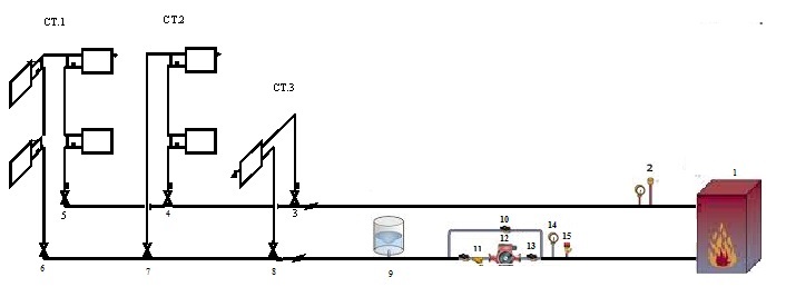
We accept a dead-end gas supply scheme. We carry out the tracing of the high-pressure inter-shop gas pipeline. We break the network into separate sections. The design scheme of the intershop gas pipeline is shown in Figure 1.1.
We determine the specific pressure losses for intershop gas pipelines:
We preliminarily determine the calculated internal diameter in the network sections:
Heat exchange devices
Efficient use of heat in rotary kilns is possible only when installing a system of in-furnace and furnace heat exchangers. Intra-furnace heat exchangers.
facade system
In order to give the reconstructed building a modern architectural appearance and radically increase the level of thermal protection of the outer walls, the system of “veins.
techno house
This style, which arose in the 80s of the last century, as a kind of ironic response to the bright prospects for industrialization and the dominance of technological progress, proclaimed at its beginning.
How to work in EXCEL
The use of Excel spreadsheets is very convenient, since the results of the hydraulic calculation are always reduced to a tabular form. It is enough to determine the sequence of actions and prepare the exact formulas.
Entering initial data
A cell is selected and a value is entered. All other information is simply taken into account.
- the value of D15 is recalculated in liters, so it is easier to perceive the flow rate;
- cell D16 - add formatting according to the condition: "If v does not fall in the range of 0.25 ... 1.5 m / s, then the background of the cell is red / the font is white."
For pipelines with a height difference between the inlet and outlet, static pressure is added to the results: 1 kg / cm2 per 10 m.
Registration of results
The author's color scheme carries a functional load:
- Light turquoise cells contain the original data - they can be changed.
- Pale green cells are input constants or data that is little subject to change.
- Yellow cells are auxiliary preliminary calculations.
- Light yellow cells are the results of calculations.
- Fonts:
- blue - initial data;
- black - intermediate/non-main results;
- red - the main and final results of the hydraulic calculation.
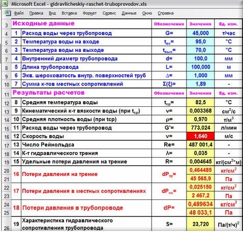
Results in an Excel spreadsheet
Example from Alexander Vorobyov
An example of a simple hydraulic calculation in Excel for a horizontal pipeline section.
- pipe length 100 meters;
- ø108 mm;
- wall thickness 4 mm.

Table of local resistance calculation results
Complicating step by step calculations in Excel, you better master the theory and partially save on design work. Thanks to a competent approach, your heating system will become optimal in terms of costs and heat transfer.