1. Hydrostatic pressure
Hydrostatic pressure is
internal compressive force due to
by the action of external forces applied to
given point in the fluid. Such pressure
in all directions is the same and depends
on the position of a point in a fluid at rest.
Dimension of hydrostatic pressure
in the MKGSS system - kg / cm2 or t / m2,
in the SI system - N/m2.
Basic unit ratios
pressure:
|
kg/cm2 |
N/m2 |
|
|
technical atmosphere |
1 |
98066,5 |
|
millimeter of water column |
0,0001 |
9,80665 |
|
millimeter of mercury |
0,00136 |
133,32 |
In practical calculations, 1 technical
atmosphere \u003d 1 kg / cm2 \u003d 10 m of water. Art. =
735 mmHg Art. = 98070 N/m2.
For an incompressible fluid that is
in balance under force
gravity, full hydrostatic
point pressure:
p=p+
 h,
h,
where p is the pressure on the free
liquid surface;
 h is the weight (gravity) of the liquid column
height h with area
cross section equal to one;
h - immersion depth
points;
 is the specific gravity of the liquid.
For some liquids, the values
specific gravity used in solving
tasks are given in the appendix (tab.
P-3).
The value of excess pressure over
atmospheric (pa)
called manometric, or
overpressure:

If the pressure on the free surface
equal to atmospheric, then excess
pressure pm=
 h.
h.
Under-atmospheric pressure
the quantity is called the vacuum:
Rwack= pa- R.
The solution to most of the problems of this
section is related to the use
the basic equation of hydrostatics

where z is the coordinate or
point mark.
1. General information on the hydraulic calculation of pipelines
When calculating
pipelines being considered
steady, uniform pressure
movement of any fluid
turbulent regime, in round-cylindrical
pipes. Fluid in pressure pipes
is under pressure and
their cross sections are completely
filled. The movement of fluid along
pipeline occurs as a result
the fact that the pressure at the beginning of it is greater than
in the end.
Hydraulic
the calculation is made in order to determine
pipeline diameter d
with a known
length to ensure skip
a certain flow rate Q
or establishing
at a given diameter and length of the required
pressure and fluid flow. Pipelines
depending on the length and pattern of their
locations are divided into simple
and complex. To simple pipelines
includes pipelines that do not have
branches along the length, with a constant
the same expense.
Pipelines
consist of pipes of the same diameter
along the entire length or from sections of pipes of different
diameters and lengths. Last case
refers to a serial connection.
Simple pipelines
depending on the length with a plot of local
resistances are divided into short and
long. short
pipelines
are
pipelines with a sufficiently short length,
in which local resistance
make up more than 10% of hydraulic
length loss. For example, they include:
siphon pipes, suction
pipes of vane pumps, siphons (pressure
water pipes under the road embankment),
pipelines inside buildings and structures
etc.
long
pipelines
called
pipelines are relatively large
lengths in which the head loss along the length
significantly outnumber local
losses. Local losses are
less than 5 10%
10%
losses along the length of the pipeline, and therefore
they can be neglected or introduced at
hydraulic calculations increasing
coefficient equal to 1.05 1,1.
1,1.
Long pipelines enter the system
water supply networks, pumping conduits
stations, conduits and pipelines
industrial enterprises and
agricultural purpose and
etc.
Complex pipelines
have different branches along the length,
those. pipeline consists of a network of pipes
certain diameters and lengths. Complex
pipelines are divided into
parallel, dead end (branched),
ring (closed) pipelines,
included in the water supply network.
Hydraulic
pipeline calculation is reduced as
usually to solve three main problems:
-
definition
pipeline flow Q,
if known
pressure H,
length l
and diameter d
pipeline,
given the availability of certain local
resistances or in their absence; -
definition
required pressure H,
necessary to secure a pass
known flow Q
by pipeline
length l
and diameter d; -
definition
pipeline diameter d
when
known head values H,
expense Q
and length l.
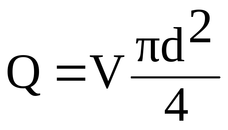
The fluid flow rate is
where q > design fluid flow, m3/s;
- area of the live section of the pipe, m2.
Friction resistance coefficient λ is determined in accordance with the regulations of the set of rules SP 40-102-2000 “Design and installation of pipelines for water supply and sewerage systems made of polymeric materials. General requirements":
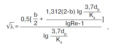
where b is some similarity number of fluid flow regimes; for b > 2, b = 2 is taken.
where Re is the actual Reynolds number.
where ν is the coefficient of kinematic viscosity of the liquid, m²/s. When calculating cold water pipes, it is taken equal to 1.31 10-6 m² / s - the viscosity of water at a temperature of +10 ° C;
Rekv > - Reynolds number corresponding to the beginning of the quadratic region of hydraulic resistance.
where Ke is the hydraulic roughness of the pipe material, m. For pipes made of polymer materials, Ke = 0.00002 m is taken if the pipe manufacturer does not give other roughness values.
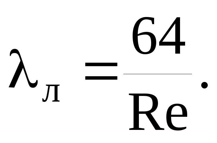
In those cases of flow when Re ≥ Rekv, the calculated value of the parameter b becomes equal to 2, and formula (4) is significantly simplified, turning into the well-known Prandtl formula:
At Ke = 0.00002 m, the quadratic resistance region occurs at a water flow rate (ν = 1.31 10-6 m²/s) equal to 32.75 m/s, which is practically unattainable in public water supply systems.
For everyday calculations, nomograms are recommended, and for more accurate calculations - "Tables for hydraulic calculations of pipelines made of polymeric materials", volume 1 "Pressure pipelines" (A.Ya. Dobromyslov, M., VNIIMP, 2004).
When calculating according to nomograms, the result is achieved by one overlay of the ruler - you should connect the point with the value of the calculated diameter on the dp scale with the point with the value of the calculated flow rate on the q (l / s) scale with a straight line, continue this straight line until it intersects with the scales of velocity V and specific losses head 1000 i (mm/m). The points of intersection of a straight line with these scales give the value V and 1000 i.
As you know, the cost of electricity for pumping liquid is directly proportional to the value of H (ceteris paribus). Substituting the expression ( 3 ) into the formula ( 2 ), it is easy to see that the value of i (and, consequently, H) is inversely proportional to the calculated diameter dp to the fifth degree.
It is shown above that the value of dp depends on the thickness of the pipe wall e: the thinner the wall, the higher dp and, accordingly, the lower the pressure loss due to friction and the cost of electricity.
If the MRS value of the pipe changes for any reason, its diameter and wall thickness (SDR) must be recalculated.
It should be borne in mind that in a number of cases the use of pipes with MRS 10 instead of pipes with MRS 8, especially pipes with MRS 6.3, makes it possible to reduce the diameter of the pipeline by one size. Therefore, in our time, the use of polyethylene PE 80 (MRS 8) and PE 100 (MRS 10) instead of polyethylene PE 63 (MRS 6.3) for the manufacture of pipes allows not only to reduce the wall thickness of pipes, their weight and material consumption, but also to reduce energy costs for pumping liquid (ceteris paribus).
In recent years (after 2013), pipes made of PE80 polyethylene have almost completely been replaced from production by pipes made of PE100 grade polyethylene. This is explained by the fact that the raw materials from which the pipes are made are supplied from abroad with the PE100 brand.And also by the fact that polyethylene 100 grade has more strength characteristics, due to which pipes are produced with the same characteristics as pipes made of PE80, but with a thinner wall, thereby increasing the throughput of polyethylene pipelines.
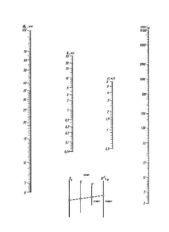
Nomogram for determining pressure losses in pipes with diameters of 6, 100 mm.
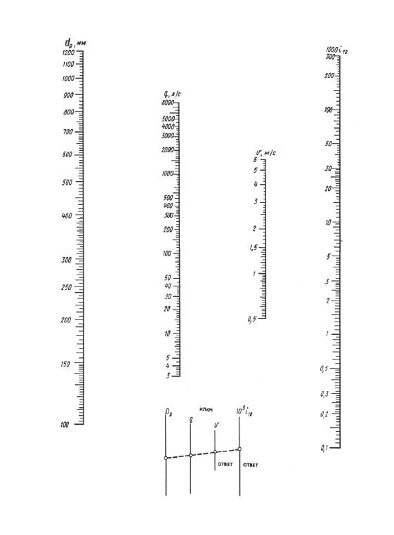
Nomogram for determining pressure losses in pipes with diameters of 100, 1200 mm.
Reynolds criterion
This dependence was brought out by the English physicist and engineer Osborne Reynolds (1842-1912).
The criterion that helps to answer the question of whether there is a need to take into account the viscosity is the Reynolds number Re. It is equal to the ratio of the energy of movement of an element of a flowing fluid to the work of internal friction forces.
Consider a cubic fluid element with edge length n. The kinetic energy of an element is:
According to Newton's law, the friction force acting on a fluid element is defined as follows:
The work of this force when moving a fluid element over a distance n is
and the ratio of the kinetic energy of the fluid element to the work of the friction force is
We reduce and get:
Re is called the Reynolds number.
Thus, Re is a dimensionless quantity that characterizes the relative role of viscous forces.
For example, if the dimensions of the body with which the liquid or gas is in contact are very small, then even with a low viscosity, Re will be insignificant and friction forces play a predominant role. On the contrary, if the dimensions of the body and the speed are large, then Re >> 1 and even a large viscosity will have almost no effect on the nature of the motion.
However, high Reynolds numbers do not always mean that viscosity does not play any role. So, when a very large (several tens or hundreds of thousands) value of the Re number is reached, a smooth laminar (from the Latin lamina - “plate”) flow turns into a turbulent one (from the Latin turbulentus - “stormy”, “chaotic”), accompanied by chaotic, unsteady movements liquids. This effect can be observed if you gradually open a water tap: a thin stream usually flows smoothly, but with an increase in the speed of water, the smoothness of the flow is disturbed. In a jet flowing out under high pressure, liquid particles move randomly, oscillating, all movement is accompanied by strong mixing.
The appearance of turbulence greatly increases the drag. In a pipeline, the turbulent flow velocity is less than the laminar flow velocity at the same pressure drops. But turbulence is not always bad. Due to the fact that mixing during turbulence is very significant, heat transfer - cooling or heating of aggregates - occurs much more intensively; the spread of chemical reactions is faster.
Bernoulli's Equation of Stationary Motion
One of the most important equations of hydromechanics was obtained in 1738 by the Swiss scientist Daniel Bernoulli (1700-1782). He was the first to describe the motion of an ideal fluid, expressed in the Bernoulli formula.
An ideal fluid is a fluid in which there are no friction forces between the elements of an ideal fluid, as well as between the ideal fluid and the walls of the vessel.
The equation of stationary motion that bears his name is:
where P is the pressure of the liquid, ρ is its density, v is the speed of movement, g is the acceleration of free fall, h is the height at which the element of the liquid is located.
The meaning of the Bernoulli equation is that inside a system filled with liquid (pipeline section) the total energy of each point is always unchanged.
The Bernoulli equation has three terms:
- ρ⋅v2/2 - dynamic pressure - kinetic energy per unit volume of the driving fluid;
- ρ⋅g⋅h - weight pressure - potential energy per unit volume of liquid;
- P - static pressure, in its origin is the work of pressure forces and does not represent a reserve of any special type of energy (“pressure energy”).
This equation explains why in narrow sections of the pipe the flow velocity increases and the pressure on the pipe walls decreases. The maximum pressure in the pipes is set exactly in the place where the pipe has the largest cross section. Narrow parts of the pipe are safe in this regard, but the pressure in them can drop so much that the liquid boils, which can lead to cavitation and destruction of the pipe material.
Navier-Stokes equation for viscous liquids
In a more rigorous formulation, the linear dependence of viscous friction on the change in fluid velocity is called the Navier-Stokes equation. It takes into account the compressibility of liquids and gases and, unlike Newton's law, is valid not only near the surface of a solid body, but also at every point in the liquid (near the surface of a solid body in the case of an incompressible liquid, the Navier-Stokes equation and Newton's law coincide).
Any gases for which the condition of a continuous medium is satisfied also obey the Navier-Stokes equation, i.e. are Newtonian fluids.
The viscosity of liquids and gases is usually significant at relatively low velocities, therefore it is sometimes said that Euler hydrodynamics is a special (limiting) case of high velocities of Navier-Stokes hydrodynamics.
At low speeds, in accordance with Newton's law of viscous friction, the drag force of the body is proportional to the speed. At high speeds, when viscosity ceases to play a significant role, the resistance of the body is proportional to the square of the speed (which was first discovered and substantiated by Newton).
Hydraulic Calculation Sequence
1.
The main circulation is selected
ring heating system (most
disadvantageously located in the hydraulic
relation). In dead-end two-pipe
systems is a ring passing through
lower instrument of the most distant and
loaded riser, in single-pipe -
through the most remote and loaded
riser.
For instance,
in a two-pipe heating system with
upper wiring main circulation
the ring will pass from the heat point
through the main riser, supply line,
through the most remote riser, heating
downstairs appliance, return line
to the heating point.
V
systems with associated water movement in
the ring is taken as the main one,
passing through the middle most
loaded stand.
2.
The main circulation ring breaks
into plots (the plot is characterized
constant water flow and the same
diameter). The diagram shows
section numbers, their lengths and thermal
loads. Thermal load of main
plots is determined by summing
thermal loads served by these
plots. To select pipe diameter
two quantities are used:
a)
given water flow;
b)
approximate specific pressure losses
for friction in the design circulation
ring RWed.
For
calculation Rcp
need to know the length of the main
circulation ring and calculated
circulation pressure.
3.
The calculated circulation
formula pressure
 ,
,
(5.1)
where
 —
—
pressure created by the pump, Pa.
System Design Practice
heating showed that the most
it is advisable to take the pressure of the pump,
equal
 ,
,
(5.2)
where
 —
—
the sum of the lengths of the sections of the main circulation
rings;
 —
—
natural pressure that occurs when
water cooling in appliances, Pa, possible
determine how
 ,
,
(5.3)
where
 —
—
distance from the center of the pump (elevator)
to the center of the device of the lower floor, m.
Meaning
coefficient possible
determine from Table 5.1.
table
5.1 - Meaning c
depending on the design temperature
water in the heating system
|
( |
|
|
85-65 |
0,6 |
|
95-70 |
0,64 |
|
105-70 |
0,66 |
|
115-70 |
0,68 |
 ),C
),C ,
, —
—
natural pressure in
as a result of water cooling in pipelines
.
V
pumping systems with bottom wiring
magnitude
 can be neglected.
-
Are determined
specific friction pressure loss
 ,
,
(5.4)
where
k=0.65 determines the proportion of pressure losses
for friction.
5.
The water consumption at the site is determined by
formula
 (5.5)
(5.5)
where
Q
- heat load on the site, W:
(tG
— tO)
- temperature difference of the coolant.
6.
By magnitude
 and
and standard pipe sizes are selected
.

6.
For selected pipeline diameters
and estimated water consumption is determined
coolant speed v
and the actual specific
friction pressure loss Rf.
At
selection of diameters in areas with small
coolant flow rates can be
big discrepancies between
 and
and .
.
underestimated losses on the
these areas are compensated by an overestimation
quantities in other areas.
7.
Friction pressure losses are determined
on the calculated area, Pa:
 .
.
(5.6)
results
calculations are entered in Table 5.2.
8.
Pressure losses in local
resistances using either the formula:
 ,
,
(5.7)
where
 - the sum of the local resistance coefficients
in the settlement area.
Meaning ξ
at each site are summarized in the table. 5.3.
Table 5.3 -
Local resistance coefficients
|
No. p / p |
Names |
Values |
Notes |
9.
Determine the total pressure loss
in every area
 .
.
(5.8)
10. Define
total pressure loss due to friction and
in local resistances in the main
circulation ring
 .
.
(5.9)
11. Compare Δр
With ΔрR.
Total pressure loss across the ring
must be less than ΔрR
on the
 .
.
(5.10)
stock of disposable
pressure is needed on unaccounted for in
calculation of hydraulic resistance.
If conditions are not
are performed, it is necessary on some
sections of the ring to change the diameters of the pipes.
12. After calculation
main circulation ring
make the linkage of the remaining rings. V
each new ring count only
additional non-common areas,
connected in parallel with sections
main ring.
Loss discrepancy
pressures on parallel connected
plots allowed up to 15% with a dead end
the movement of water and up to 5% - with passing.
table
5.2 - Results of hydraulic calculation
for heating system
|
On the |
By |
By |
||||||||||||||
|
Number |
Thermal |
Consumption |
Length |
Diameter |
Speed |
Specific |
Losses |
Sum |
Losses |
d, |
v, |
R, |
Δрtr, |
∑ξ |
Z, |
Rl+Z, |
Lesson 6
Change in gas temperature along the length of the gas pipeline
In stationary gas flow, the mass
the flow rate in the gas pipeline is
 . (2.41)
In fact, the movement of gas in the gas pipeline
is always non-isothermal. V
During compression, the gas heats up.
Even after its cooling at the COP, the temperature
gas entering the pipeline
is about 2040С,
which is much higher than the temperature
environment (T).
In practice, the temperature of the gas becomes
close to ambient temperature
only for gas pipelines of small diameter
(Dy0.
Moreover, it should be taken into account that
pipelined gas
is a real gas, which is inherent
the Joule-Thompson effect, which takes into account
absorption of heat during gas expansion.
When the temperature changes along the length
gas pipeline gas movement is described
system of equations:
specific energy ,
,
continuity ,
,
states ,
,
heat balance .
.
Consider in the first approximation the equation
heat balance without taking into account the effect
Joule Thompson. Integrating the equation
heat balance
 ,
,
we get
 , (2.42)
where ;
;
KSR- average on the site full
heat transfer coefficient from gas to
environment;
G is the mass flow rate of gas;
cP–
average isobaric heat capacity of the gas.
a valuetL is called the dimensionless criterion
Shukhov
 (2.43)
So the gas temperature at the end
gas pipeline will be
 . (2.44)
At a distance x from the beginning
gas pipeline gas temperature is determined
according to the formula
 . (2.45)
Change in temperature along the length of the gas pipeline
is exponential (Fig.
2.6).
Consider
effect of gas temperature change on
pipeline performance.
Multiplying both sides of the specific equation
energy on 2 and expressing ,
,
we get
 . (2.46)
We express the density of the gas on the left side
expressions (2.46) from the equation of state
 ,
,
productwfrom the continuity equation ,dx from the thermal
balance .
.
With this in mind, the specific equation
energy takes the form
 (2.47)
or
 . (2.48)
Denoting
 and integrating the left side of the equation
(2.48) from PHdoPTO, and to the right from THdoTTO, we get
 . (2.49)
By replacing
 , (2.50)
we have
 . (2.51)
After integrating in the specified
limits, we get

 . (2.52)
Taking into account (2.42)

or
 , (2.53)
where is a correction factor that takes into account
temperature change along the length of the gas pipeline
(non-isothermality of the gas flow).
Taking into account (2.53), the dependence for determining
mass flow rate of gas will take the form
 . (2.54)
Value Halways greater than one, so
mass flow rate of gas when changing
temperature along the length of the gas pipeline
(non-isothermal flow regime) always
less than in isothermal mode
(T=idem). Product THis called the mean integral
temperature of the gas in the pipeline.
With the values of the Shukhov number Shu4
gas flow in the pipeline
consider almost isothermal
at T=idem. Such a temperature
mode is possible when pumping gas with
low gas pipeline costs
small (less than 500 mm) diameter to a significant
distance.
Effect of changing gas temperature
manifests itself for the values of the Shukhov number
Shu
At
gas pumping the presence of a throttle
effect leads to a deeper
gas cooling than only with heat exchange
with soil. In this case the temperature
gas can even drop below
temperature T (Fig.
2.7).
Rice. 2.7. Influence of the Joule-Thompson effect
on the gas temperature distribution over
pipeline length
1 - without taking into account Di; 2 - with
taking into account Di
Then, taking into account the Joule-Thompson coefficient
law of temperature change along the length
takes the form
 , (2.55)
5 Hydraulic losses
Difference
oil pressure in two sections of one
and the same pipeline, provided that
the first is located upstream, and
the second - below, is determined equation
Bernoulli
 ,
,
where
h2
– h1
- the difference in the heights of the centers of gravity
sections from an arbitrarily chosen
horizontal level;
v1,
v2
– average speeds of oil in sections;
g - force acceleration
gravity;
 -sum
-sum
hydraulic losses during movement
oils from the first section to the second.
The equation
Bernoulli in full use
for calculation of suction lines of pumps;
in other cases, the first term,
usually neglected and considered:

hydraulic
losses are usually divided into local
losses and friction losses along the length
pipelines (linear).
1.5.1
local losses
energies are due to local
hydraulic resistance,
causing flow distortion. Local
resistances are: constrictions,
expansion, rounding of pipelines,
filters, control equipment and
regulation, etc. When flowing
liquids through local resistances
its speed changes and usually there are
large vortices.
Losses
pressure from local resistances
determined by the formula Weisbach:
 MPa
MPa
(or
 Pa),
Pa),
where
 (xi) – drag coefficient or
loss,
v
is the average flow velocity over the cross section
in a pipe behind local resistance, m/s;
,
N/m3;
g=9.81 m/s2.
Each
local resistance is characterized
by its coefficient value
 .
.
With turbulent flow, the values determined mainly by the form of local
resistance and change very little
with a change in the size of the section, speed
fluid flow and viscosity. So
assume that they do not depend on the number
Reynolds Re.
Values
 ,
,
for example, for tees with the same
channel diameters are taken equal,
if:
streams
add up, diverge; flow
passing;
 =0,5-0,6
 =1,5-2
 =0,3
=0,3 =1-1,5
 =0,1
=0,1 =0,05
=0,05

 =0,7
=0,7
 =0,9-1,2
 =2
=2
at
pipe bend
 = 1.5-2, etc.
Values
 for specific resistances encountered
in hydraulic systems of equipment, taken from
reference literature.
At
laminar flow (Re
Losses
pressure from local resistances at
laminar flow are determined by
formula:
 MPa
MPa
where
 l
l
= a and laminar correction factor
Quantities
pressure loss in standard
hydraulic devices for
nominal flow rate usually
listed in their technical specifications.
1.5.2
Loss on
length friction
is the energy loss that occurs
in straight pipes of constant cross section,
those. with uniform fluid flow,
and increase in proportion to the length
pipes. These losses are due to internal
friction in a liquid, and therefore have
place in both rough and smooth pipes.
Losses
pipeline friction pressure
is determined by the formula Darcy:
 MPa
MPa
where
 is the coefficient of friction in the pipeline;
l
and d
- length and internal diameter of the pipeline,
mm.
This
the formula is applicable both for laminar,
as well as in turbulent flow; difference
consists only in the values of the coefficient
 .
.
At
laminar flow (Re
At
turbulent flow coefficient of friction
is not only a function of Re, but
also depends on the roughness of the internal
pipe surface. For hydraulically
smooth pipes,
those. with a roughness that
practically does not affect its resistance,
turbulent friction coefficient
mode can be determined by the formula PC.
Konakova:

pipe
is considered hydraulically smooth if
(d/k)>(Re/20),
where k is the equivalent roughness,
mm. For example, for new seamless steel
pipes k≈0.03
mm, and after several years of operation
k≈0.2
mm, for new seamless pipes made of
non-ferrous metals k≈0.005
mm. These pipes are often used in
hydraulic systems of machine tools.
Coefficient
friction in the turbulent regime can be
determine by formula Altshulya,
being universal (i.e. applicable
in any case):

2. Flow characteristics of the pipeline flow module
Let's remember
linear loss formula - Darcy formula
- Weisbach:
 .
.
Express
in this formula, the speed V
through flow Q
from the relation
 :
:
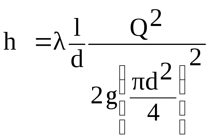 .
.
(6.1)
For
pipeline of a certain diameter
complex of quantities
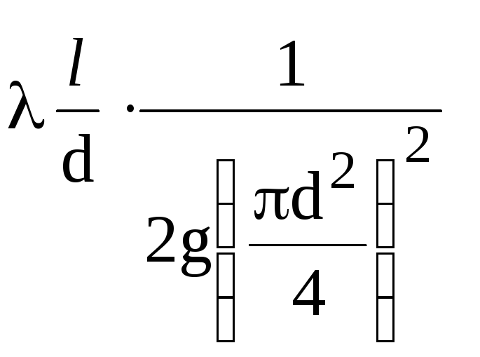 in expression (6.1) can be considered as the quantity
constant (1/K2),
except for the hydraulic coefficient
friction λ. Based on the concept
average economic speed Vs.e
let us show that the indicated coefficient λ
can be attributed to this complex, because v
In this case, the Reynolds number will be
have a specific meaning:
 ,
,
and on the Nikuradze plot, the coefficient λ in
this case will have a specific
meaning.
Justify
legitimacy of introducing the concept
average economic speed as follows
reasoning.
hydraulic
system, such as plumbing,
you can skip a certain expense
made from pipes of different diameters. At
At the same time, with an increase in the diameter d,
therefore, a decrease in the speed V
capital expenditures will rise, and
operating costs will
decrease due to a decrease in hydraulic
losses. The speed at which the total
costs will be minimal
will be called the average economic
speed Vs.e
= 0.8 ... 1.3 m / s (Fig. 6.1).
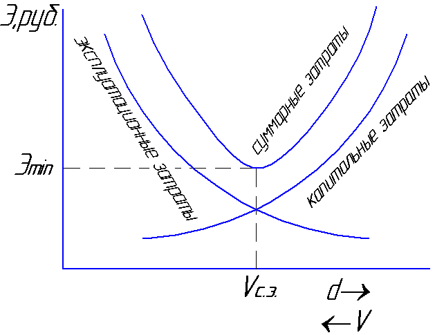
fig.6.1
Then
the linear loss formula (6.1) takes the form
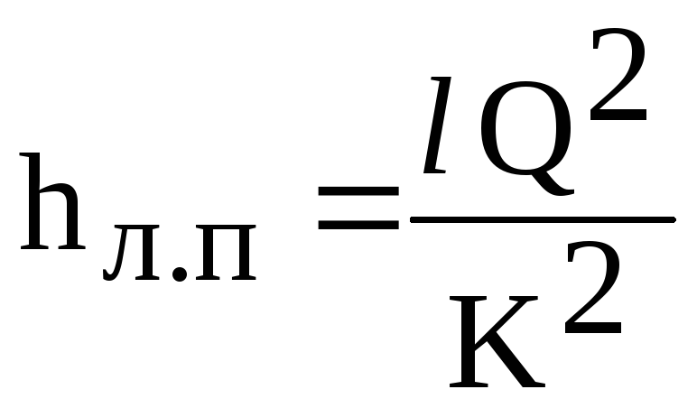 ,
,
(6.2)
where
K - flow characteristic of the pipeline
(flow modulus), dependent on material
pipeline, diameter and flow. is taken
from tables.